(2,-3).jpg)
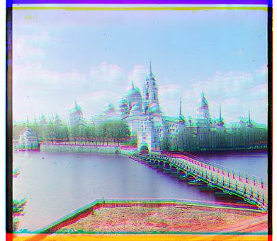
The aim of this project was to align three pictures which were taken by Sergei Mikhailovich Prokudin-Gorskii where each picture had been taken with a red, green and blue filter. The result would then resemble a "normal" color photo. All of the results are presented at the bottom of the page. The shifts are presented under the images in the following order: Red (x,y), Green (x,y).
The first task was to align the jog images which had a significantly lower resolution. For these low resolution images a brute force search was suggested by the project instructions using either SSD (Sum of squared differences) or NCC (Normalized cross correlation). An SSD implementation was computationally slightly quicker and was therefore used throughout the rest of the project and NCC was discarded. The SSD implementation uses a [-15,15] window where every pixel in the images are compared to each other using SSD where there aim is to minimize SSD between the pixels. If a lower SSD is found the image then rolls using np.roll(). The results were better but not very good. I came to realization that it might be because of the borders of the image. I therefore opted to manually crop all of the images 10% on every side. This resulted in a much better shift and final image. This was not optimal however and I therefore decided to keep the original images but instead make the searches and comparisons in a cropped image while keeping the original one for the output. This yielded the same result as for the cropped image but without actually cropping it. The result of one of the images along with the displacement in x and y are presented down below, the rest are presented at the bottom of the page.

(2,-3).jpg)
The next part was to use some sort of image pyramid to align the larger .tif images. Using simply SSD was not viable
from a computation time standpoint since the window for pixels which would need to be compared would have to be significantly
larger than [-15,15], hence the need for a pyramid. I created a Gaussian pyramid by doing the following:
First a list to
add the images to was created where the original image was added. Then the original image was blurred using
cv2.GaussianBlur() and thereafter downsampled to half of the original image size by slicing the image. This new image was then added to the
list and this process was then repeated four times which resulted in a total of five layers in the pyramid, including the
original. For example, church.tif original size was 3202x3634 where the most downsampled layer in that pyramid was
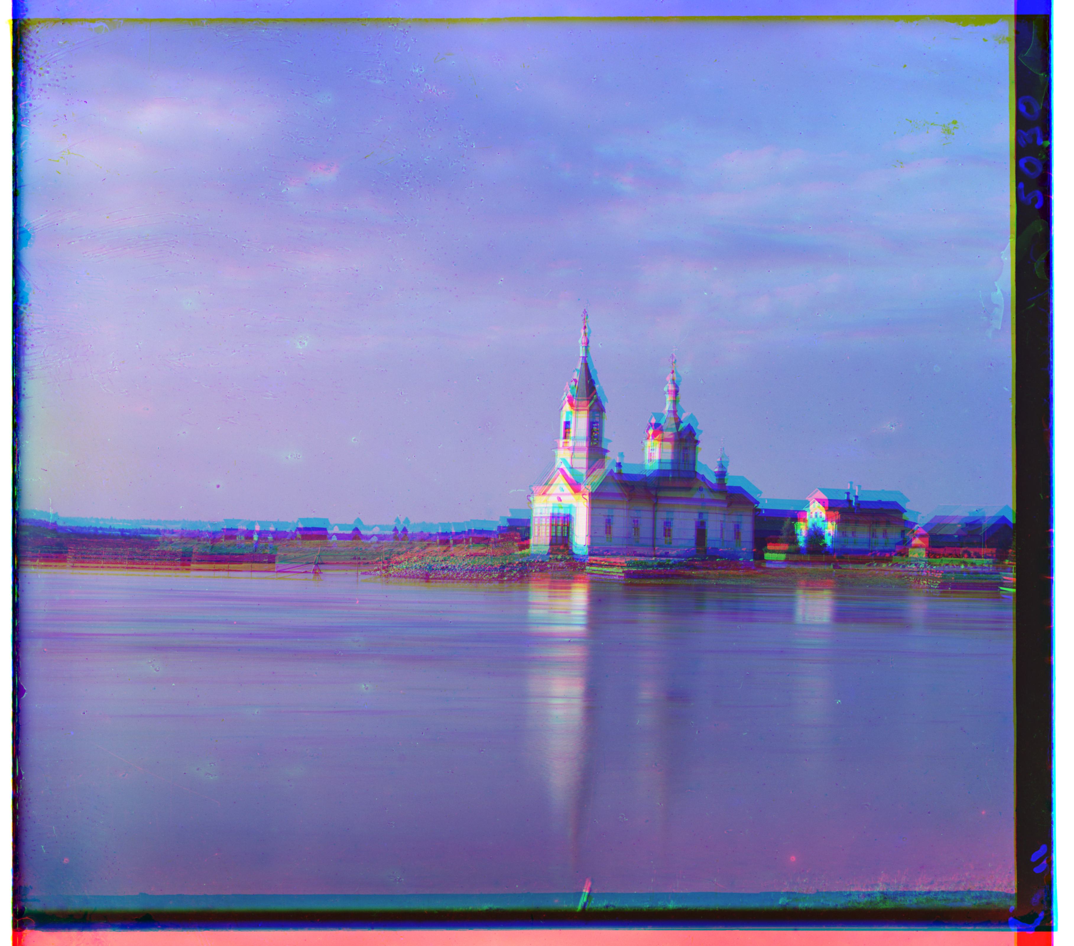
201x228. The search was done using a recursive method. The alignment starts with the most downsampled image with a search window
of [-32,32] and is decreased by half for every layer you go up in the pyramid. The displacement is also scaled by two every time
you go to a different layer to keep the proper proportions. Assuming that the images are relatively well aligned after two
alignments, there is not really any need for a large search window and thus a lot of computation time can be saved. The result
of one of the images along with the displacement in x and y are presented down below, the rest are presented at the bottom of the
page.
(3,25).jpg)
Simply using the gaussian pyramid for alignment did not work very well for emir.tif. Therefore I tried to identify the edges and using that to get a better alignment. Edge detection was made using cv2.Canny(). This was then incorporated in the SSD function. This yielded a much better result on the emir and a slightly better result for the other images. Before edge detection and after after edge detection for the emir is presented down below.
(24,49).jpg)
(24,49).jpg)
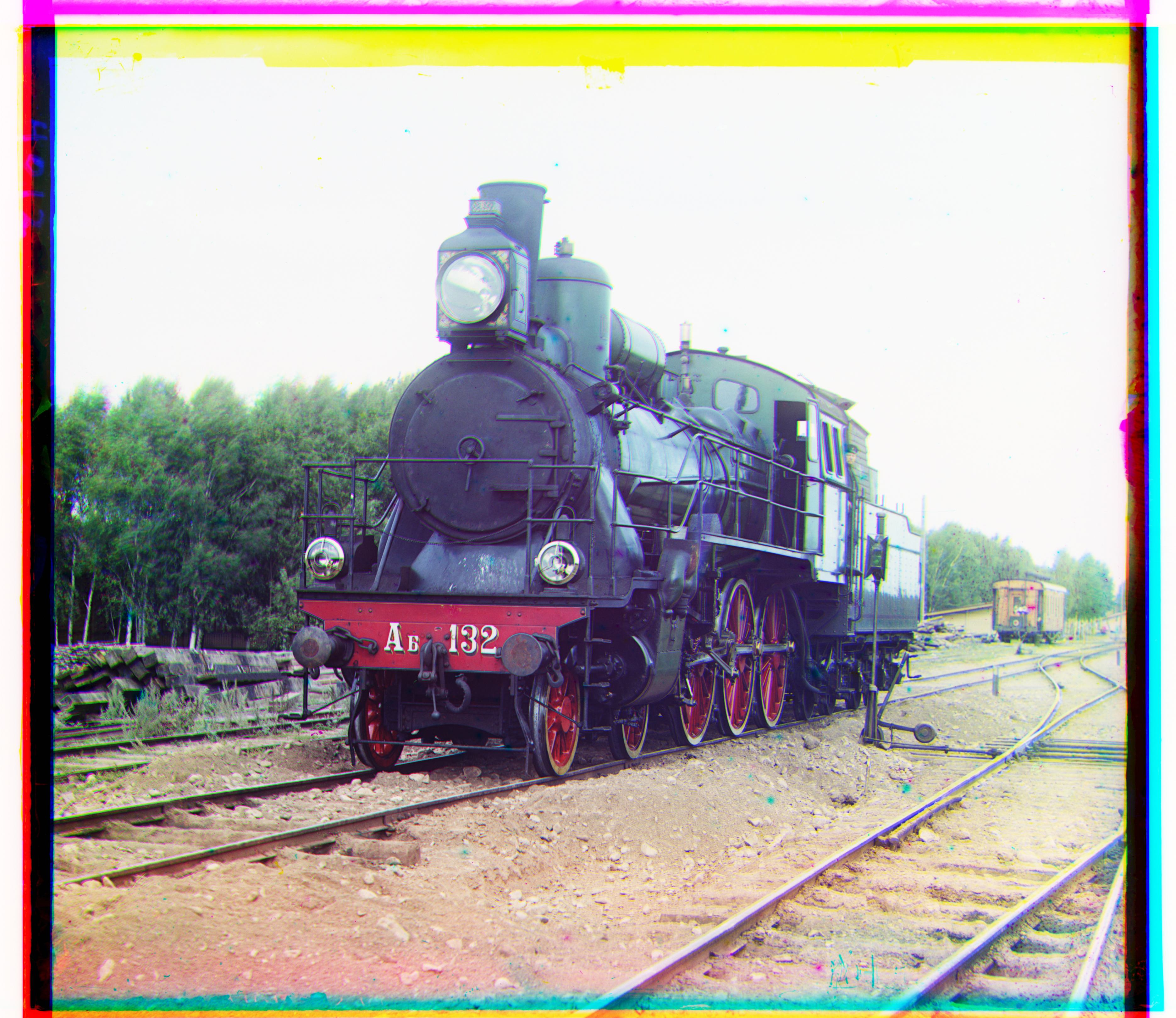
I tried to implement automatic white balance for the images by setting the brightest pixel of the image to be the brightest possible pixel (value 1.0) and using that as a reference to scale the other pixels. It doesn't seem to make too much of a difference though.
(0,44).jpg)
(3,25).jpg)
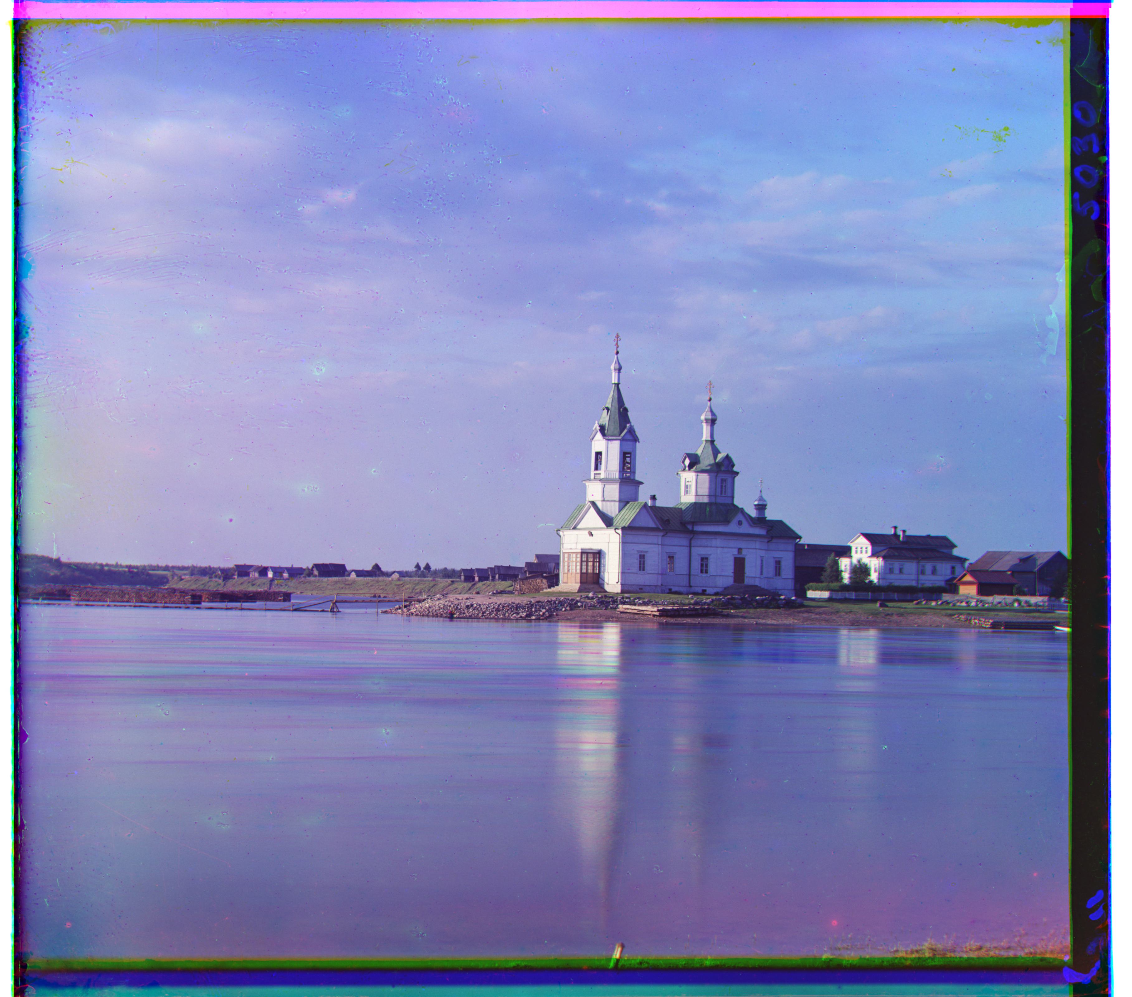
Since the automatic white balance didn't do too much I tried to implement it using the gray-world assumption. I did so by taking the mean of all the pixel values in every color channel and then taking the mean of these three which resulted in a total average. Then each color channel was scaled by multiplying the color channel with the total average and dividing with the color channel's mean. This yielded a more noticeable difference. Some of the results are presented down below.
(24,49).jpg)
(24,49).jpg)
(0,44).jpg)
(0,44).jpg)
(3,25).jpg)
(4,24).jpg)
(2,5).jpg)
(4,24).jpg)
(24,49).jpg)
(17,60).jpg)
(16,39).jpg)
(10,56).jpg)
(10,80).jpg)
(2,-3).jpg)
(24,52).jpg)
(-11,33).jpg)
(29,77).jpg)
(16,56).jpg)
(2,3).jpg)
(0,44).jpg)