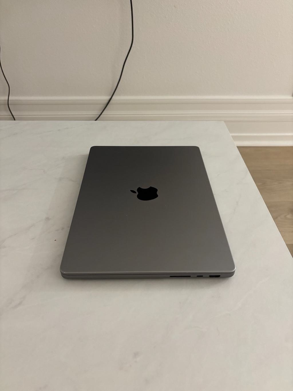
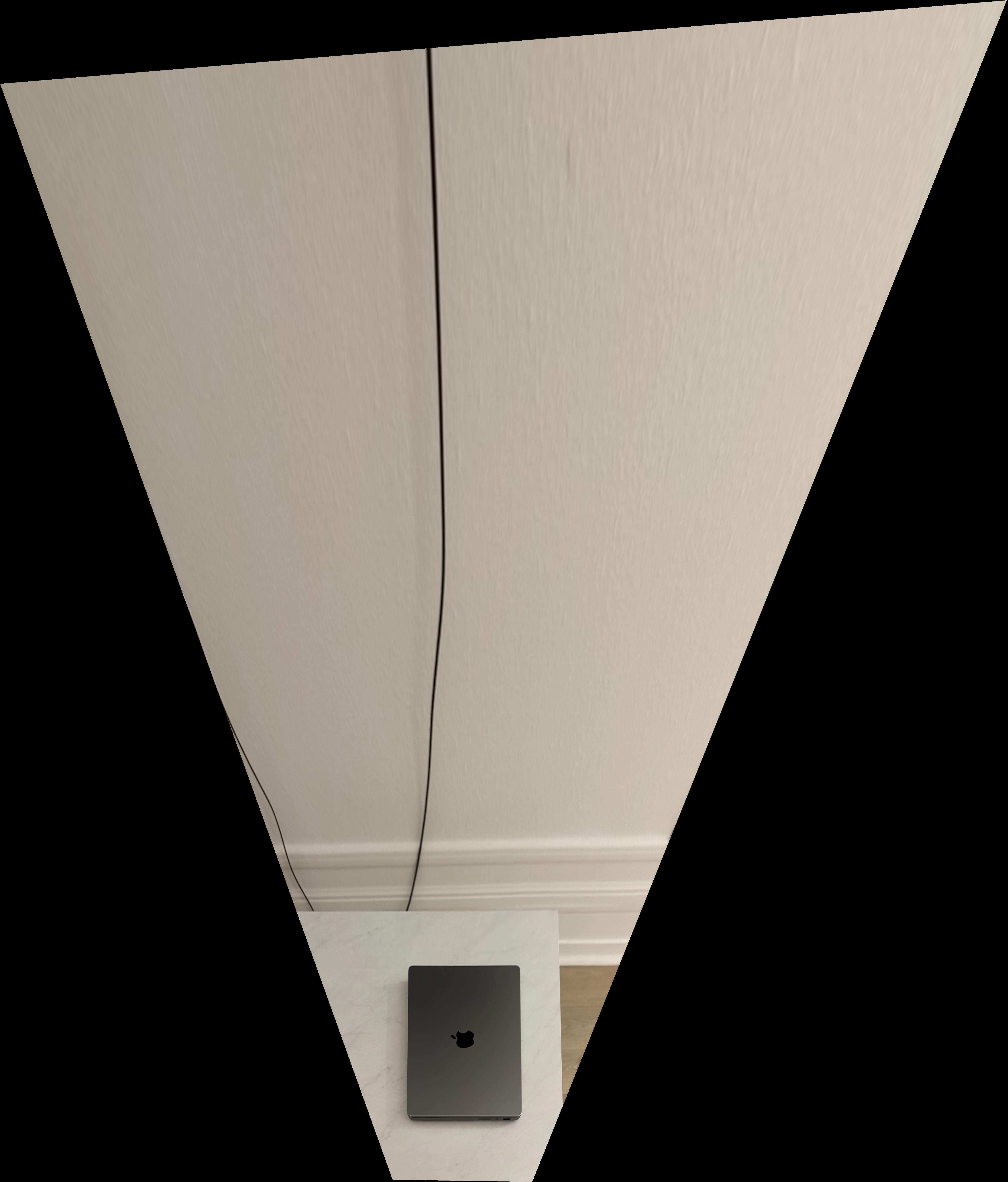
The goal of this project was to warp images and change their perspective and subsequently create a panoramic looking image.
The computeH function calculates the homography matrix \( H \) that maps points from one image to another using
corresponding point pairs. These correspondences were made using the provided online tool.
For each point pair \( (x_1, y_1) \) in im1_pts and \( (x_2, y_2) \) in im2_pts, we append two rows to matrix \( A \):
$$ \begin{pmatrix} x_1 & y_1 & 1 & 0 & 0 & 0 & -x_1 x_2 & -y_1 x_2 \end{pmatrix} $$ $$ \begin{pmatrix} 0 & 0 & 0 & x_1 & y_1 & 1 & -x_1 y_2 & -y_1 y_2 \end{pmatrix} $$
We solve for \( h \) using least squares and reshape it into the final homography matrix:
$$ H = \begin{pmatrix} h_{11} & h_{12} & h_{13} \\ h_{21} & h_{22} & h_{23} \\ h_{31} & h_{32} & 1 \end{pmatrix} $$
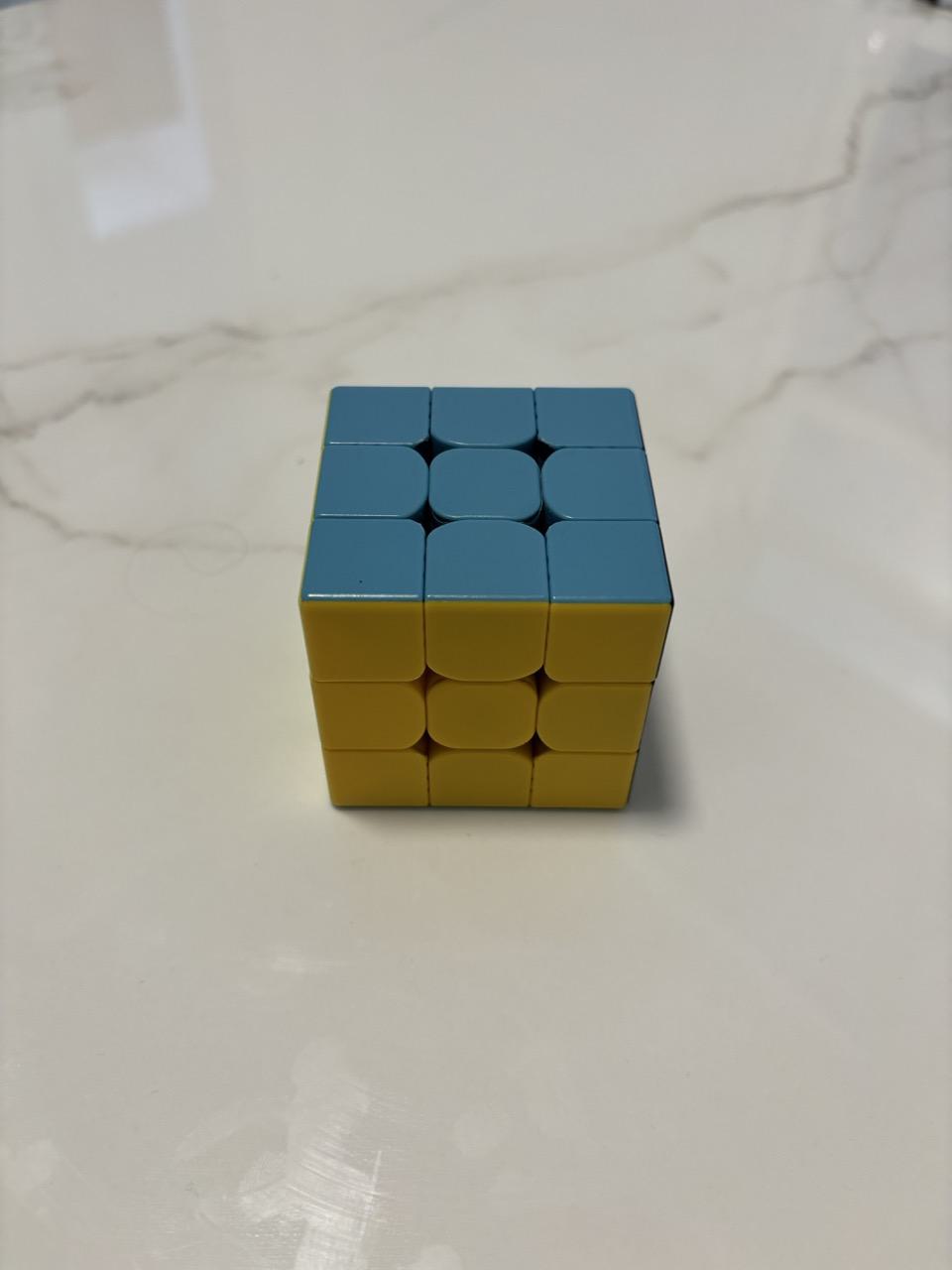
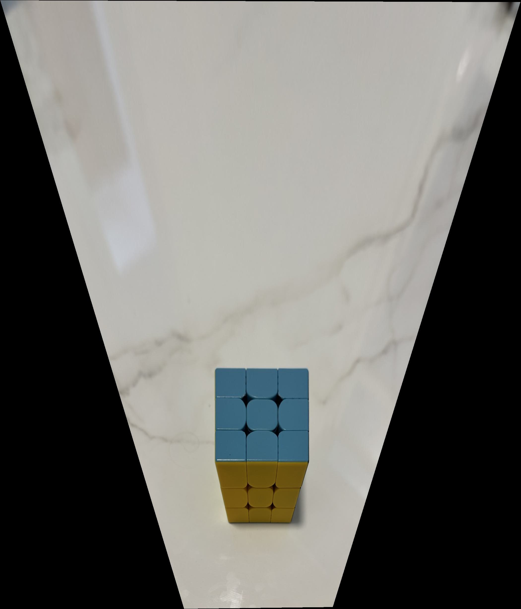
The next step was to use the homography to rectify images. This was done by taking a picture if something, slightly skewed. Then points were selected using the online tool. With the computed homography, the image could then be warped by mapping the keypoints to the new location. The warping was done using an inverse warp along with some interpolation. The results are presented down below.


The mosaic blending process combines two images into one by warping one image to align with the other and creating a transition between them. The steps involved are as follows:
The first image is transformed using a homography matrix, which aligns it with the perspective of the second image. After warping, the bounding box for both images is determined. This ensures the final output can hold both images by calculating the minimal and maximal coordinates of the two images.
Two empty images are created, large enough to contain both the warped and non-warped images. The warped image is placed into the first image, and the non-warped image is placed into the second image, with correct offsets applied to ensure proper alignment. This was by far the most time consuming and frustrating part of this project.
A blending mask is generated to handle the transition between the two images. This is done by creating binary masks of the non-empty regions of both images. Then, the distance of each pixel from the nearest edge is calculated to create a gradual transition between the two images. The distances are normalized to produce a transition mask, which determines how the two images will blend together.
The blending mask is applied to both images, ensuring that the two images transition in the overlapping region. The pixels from each image are combined based on the values of the mask, resulting in a blend where the images overlap.
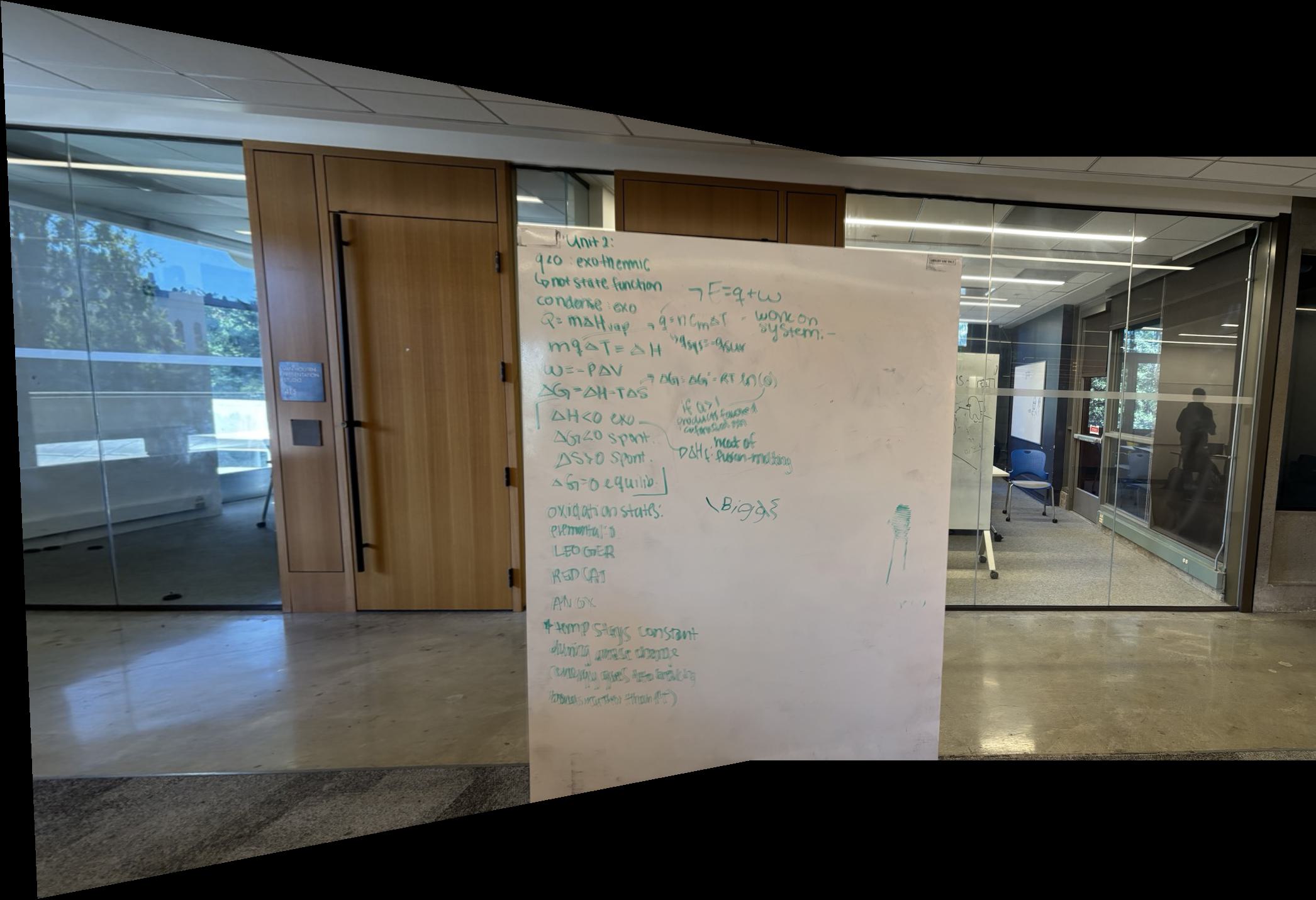
The final mosaic is created by combining the two images into one, with a transition in the overlapping regions, producing a visually cohesive result without too many noticeable artifacts.
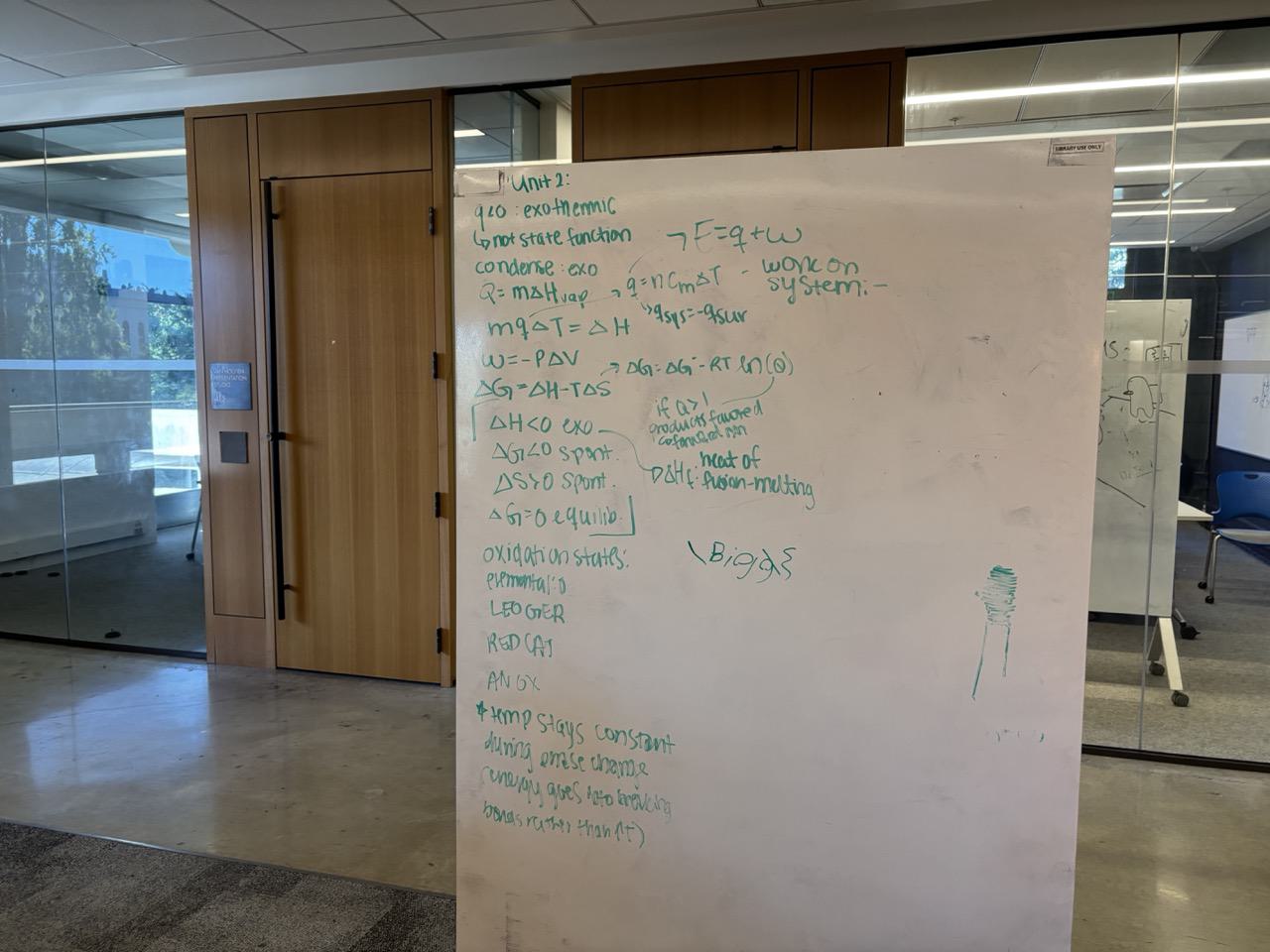
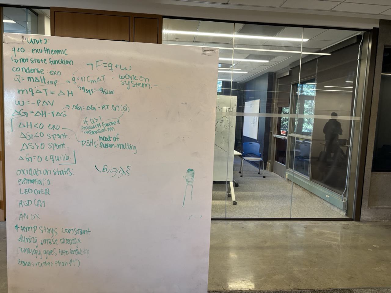
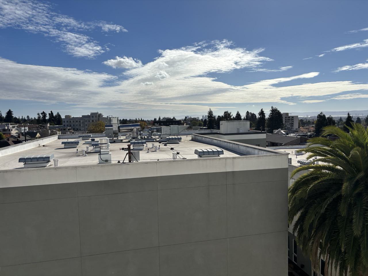
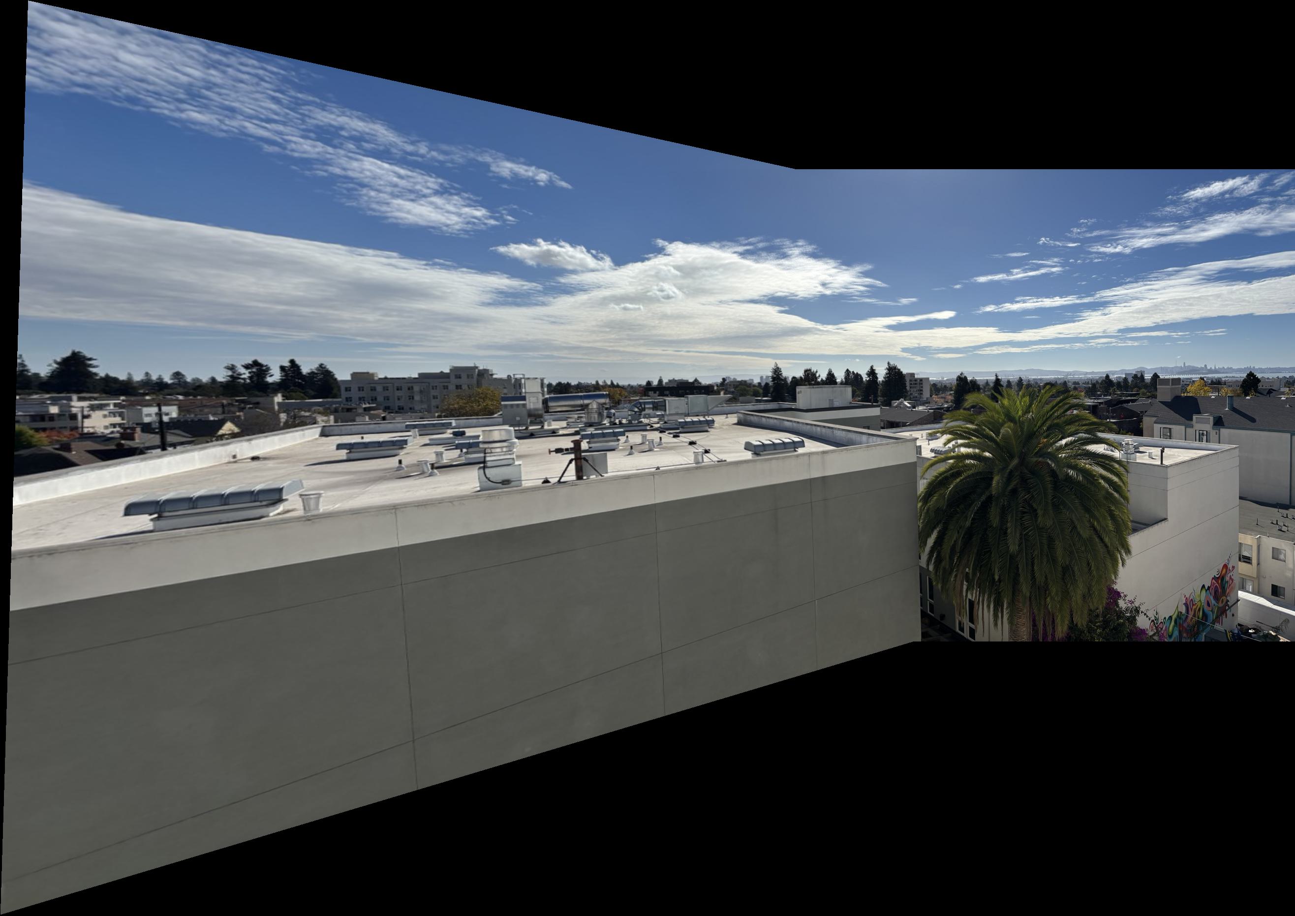
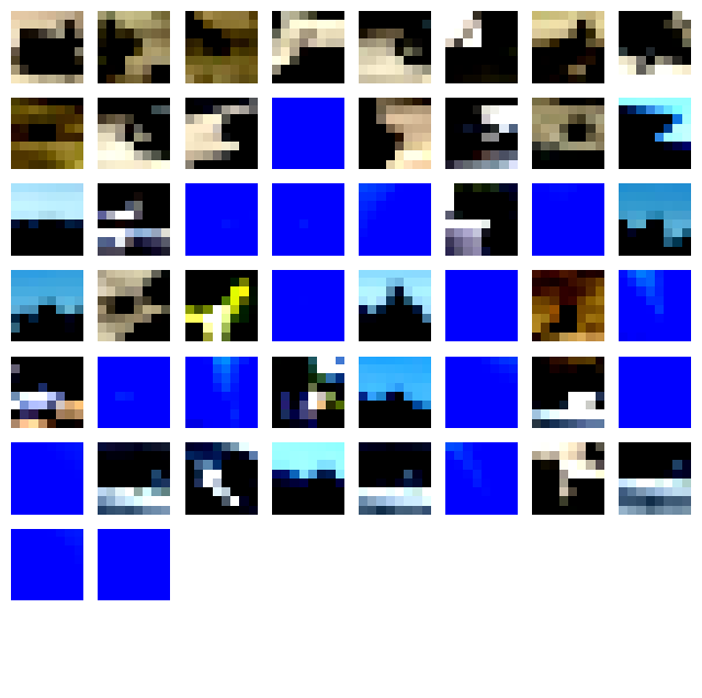
Three different mosaics were created. There are still some small artifacts left. In the mosaic of my room, the exposure in the two images were quite different and therefore the blending was not perfect. In the other two mosaics you can see some slight blurring where the images are stitched together. But all in all, an ok result in my opinion. The source images and the results are presented down below.
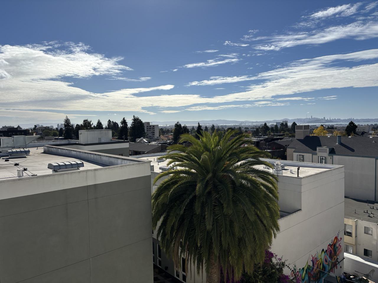
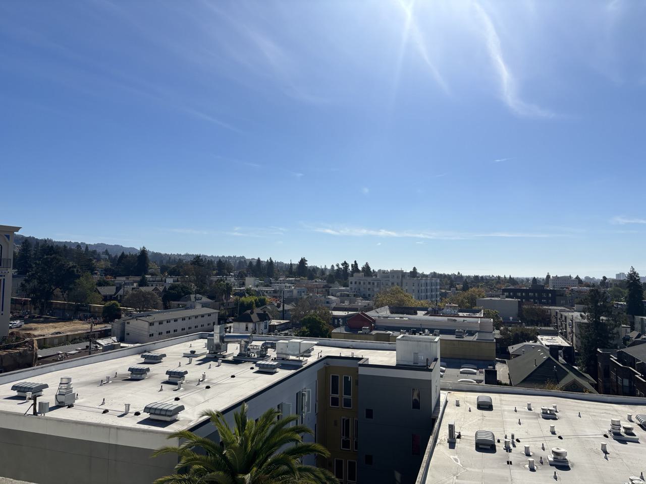
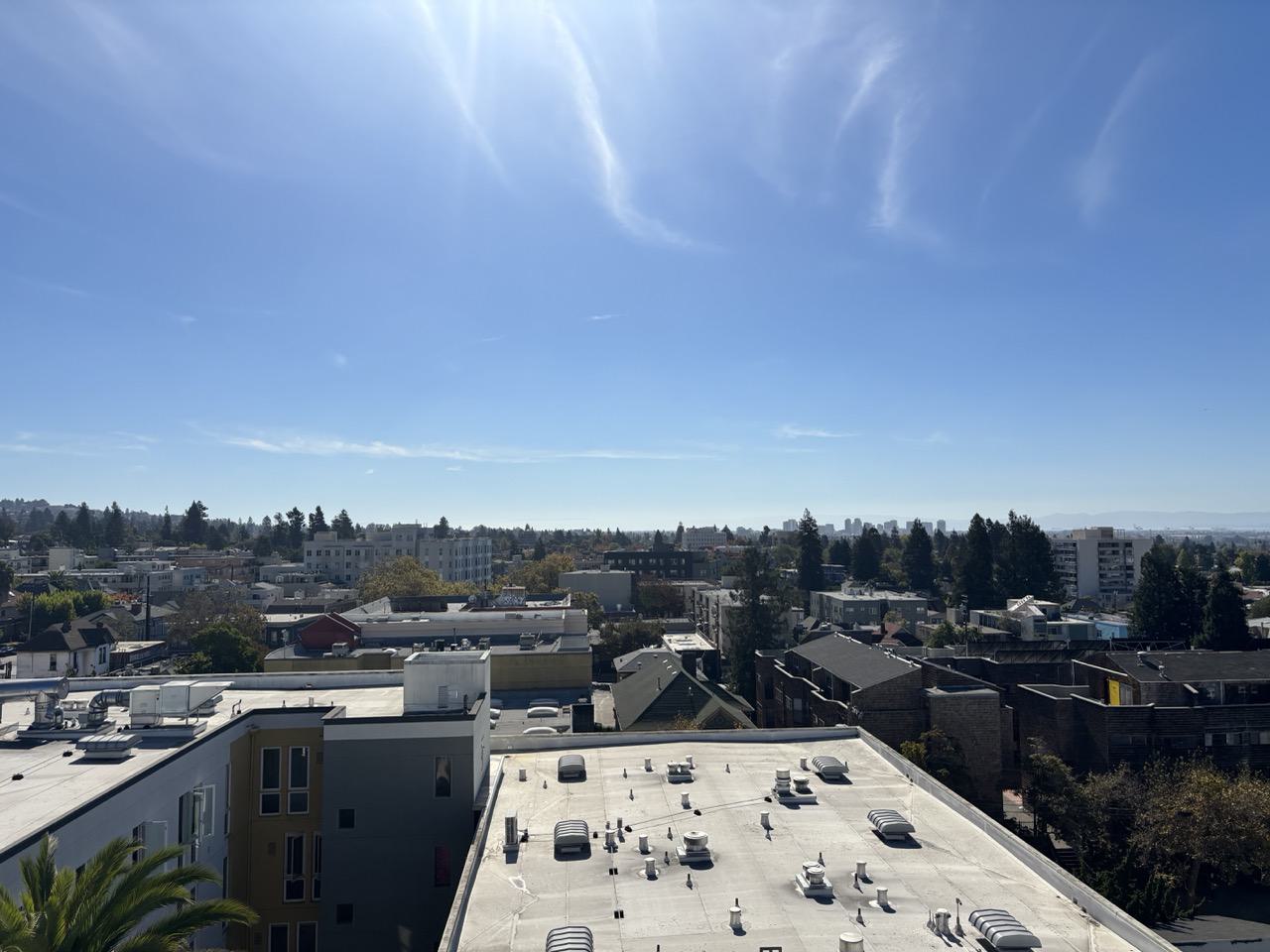
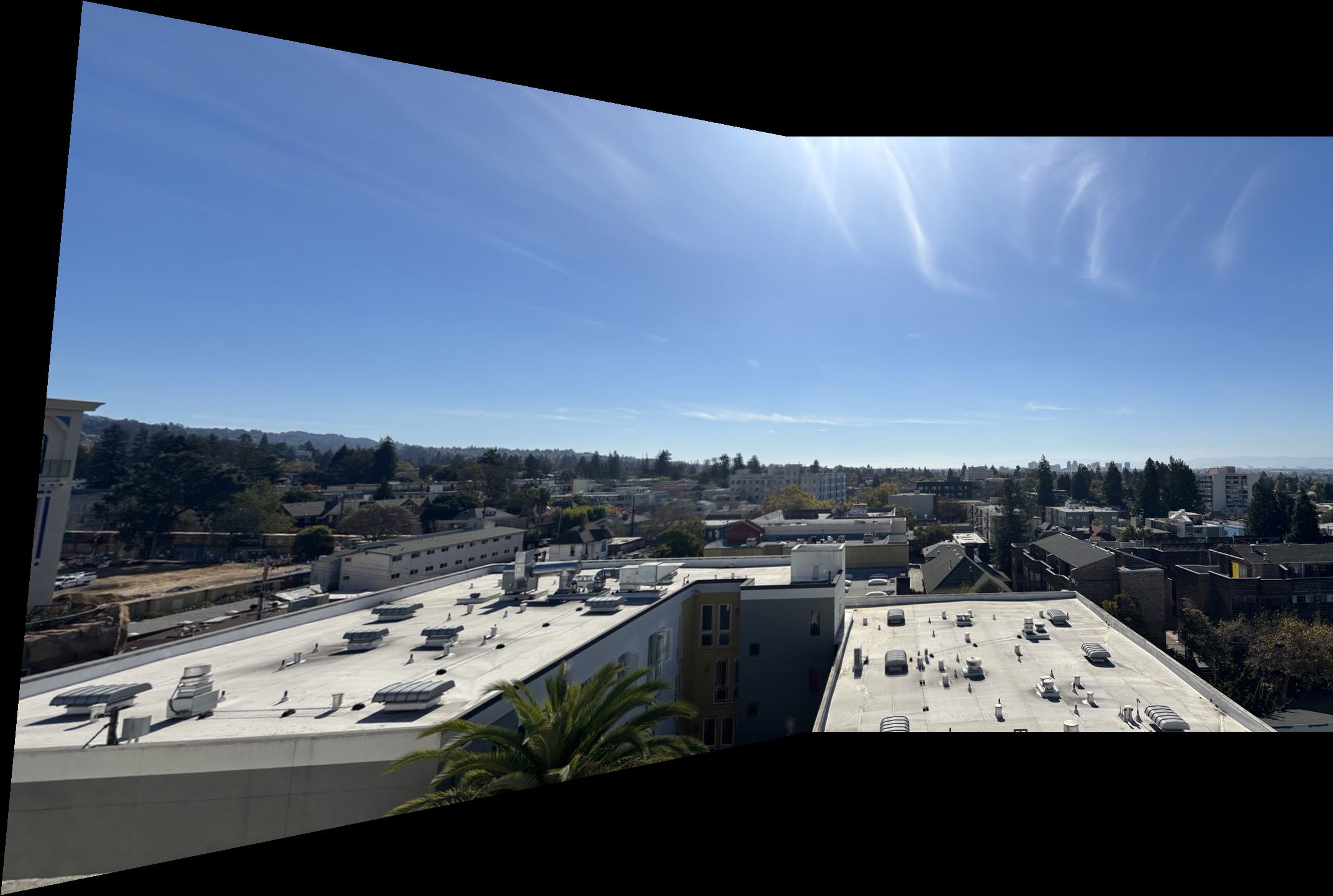
First, the given code for Harris corner detection was run in order to compute the interest points in the image. These interest points were way too many which is displayed below.
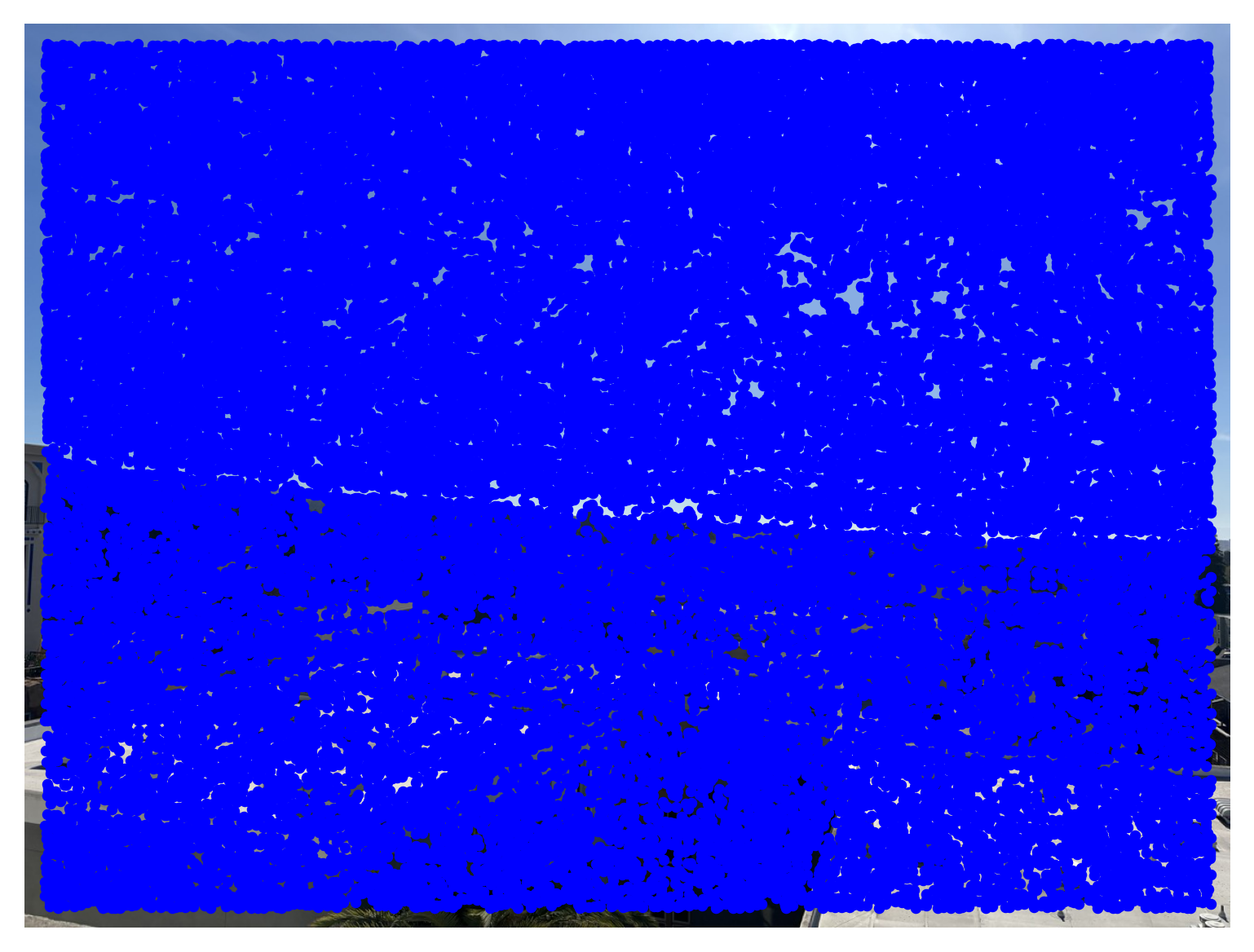
This approach uses the adaptive non-maximal suppression (ANMS) algorithm to select well-separated interest points. It calculates a distance, \( r_i \), for each interest point \( \vec{x}_i \) to its nearest point \( \vec{x}_j \) with a significantly higher corner response. Specifically, it finds the minimum distance to any \( \vec{x}_j \) such that \( h(\vec{x}_i) < c_{\text{robust}} \cdot h(\vec{x}_j) \). Only the top-K points with the largest \( r_i \) values are kept, ensuring that interest points are not clustered together but spread evenly across the image. The result is displayed below.
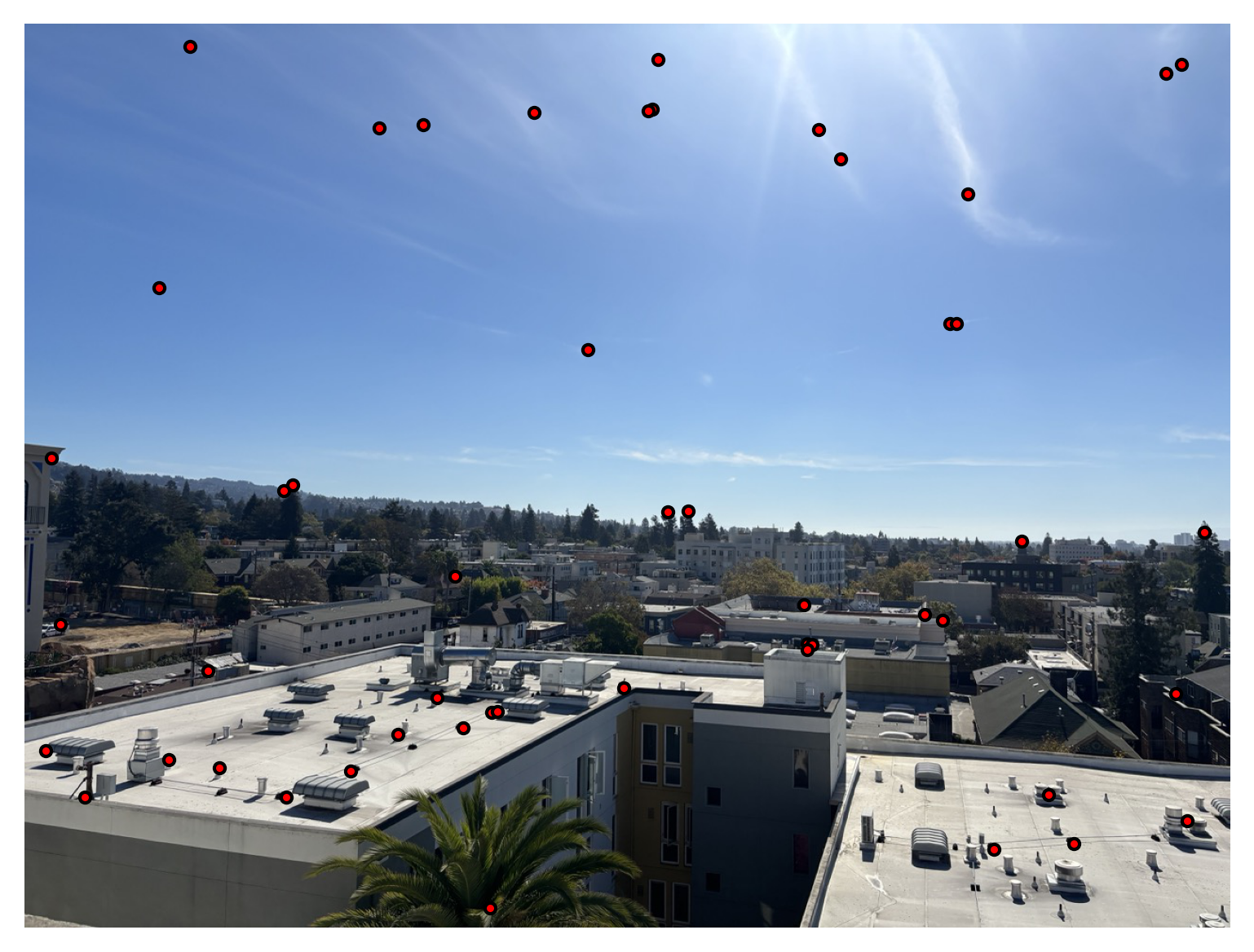
Using the calculated interest points, feature patches were extracted for each points. Patches were taken around specific interest points in the image. Each patch was centered on the point and sized to avoid interference from edge effects. To standardize the patches, their intensity values were normalized by adjusting for mean and variance, ensuring consistent contrast. Each patch was then resized to a smaller, uniform scale, making the data compact and optimized for subsequent processing and comparison. The patches are displayed below.
Having the feature extraction in place, it was now time to match features in two images. For each patch in the first image, distances to patches in the second were calculated based on the sum of squared differences (SSD). To ensure reliable matches, Lowe's ratio test was applied, comparing the closest and second-closest matches for each feature. This filtering step helped retain only robust matches, which were then output as corresponding coordinates in both images. The result is displayed below.
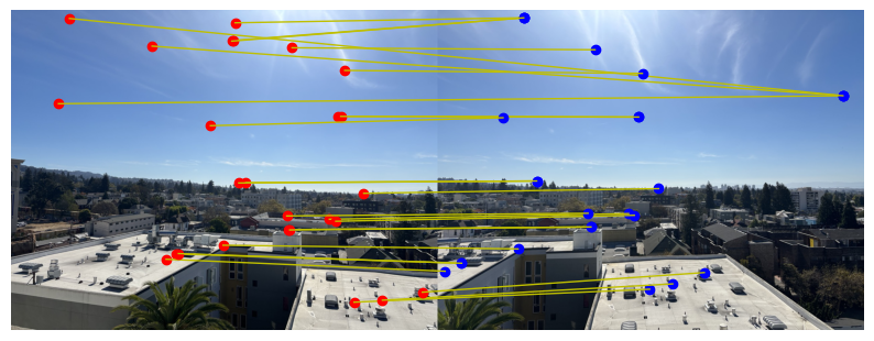
The feature matching may seem solid but there can still be outliers present. Therefore we turn to RANSAC - Random sample consensus. This is used to ensure a robust transformation by handling outliers in the matched points. By iteratively selecting random subsets of matches to compute possible homographies, RANSAC identifies the transformation with the most inliers, discarding mismatches. This approach yields an accurate homography that aligns the images, even when only a subset of matches is correct. The difference when using RANSAC and not is displayed below.


The results for the manual mosaicing and the "automatic" keypoint detection and stitching are displayed alongside each other down below.

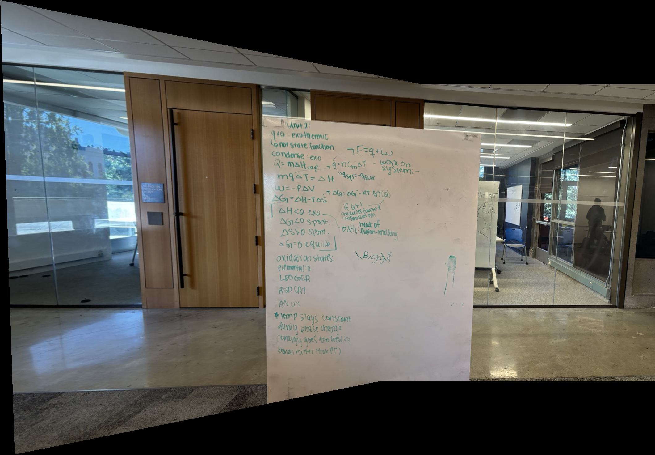

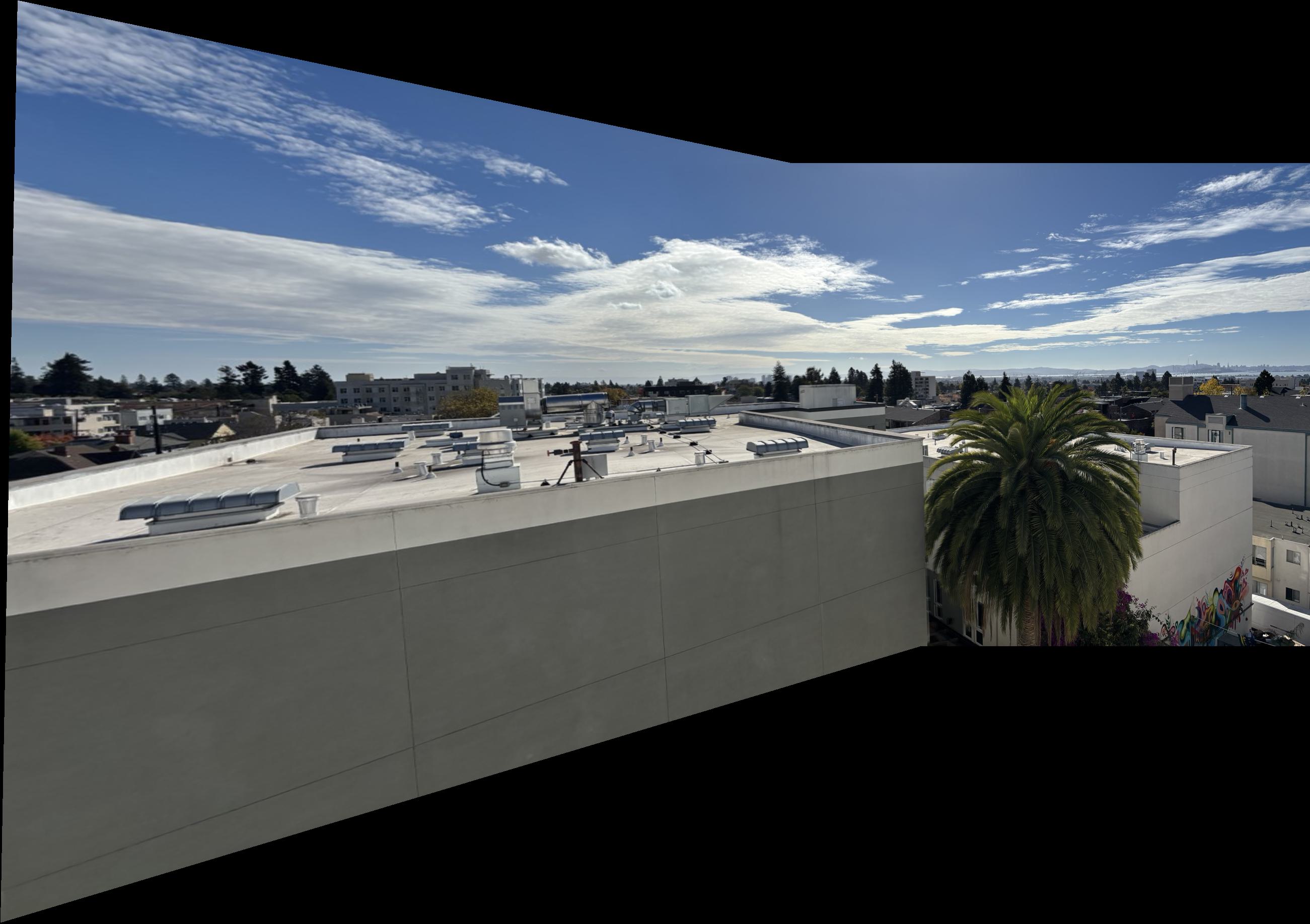

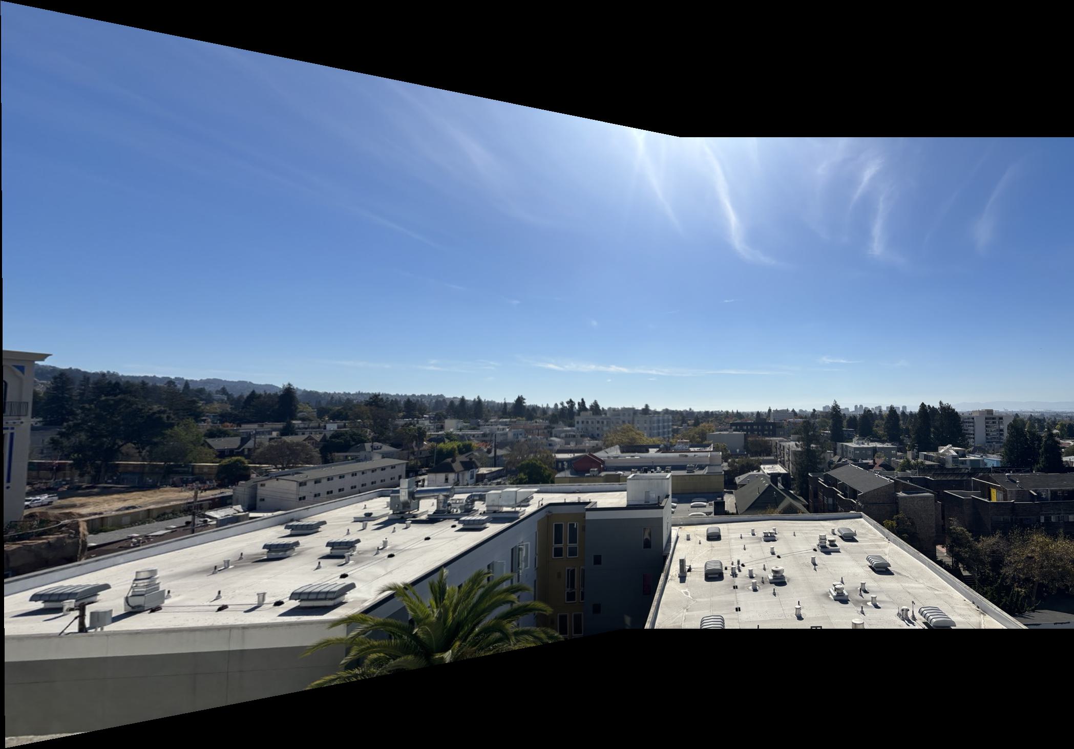
There are some slight differences but the overall result is largely the same. In then first mosaic there is some blurring at the bottom where the images are stitched. This is better in the automated one. The same goes for the last mosaic where some blurring occurs at the seam in the manual one where the automatic one handles it better. The automatic corner detection, stitching etc. is thus in my opinion, deemed successful. The coolest thing about this project for me is the automatization of processes. Being able to choose the correct keypoints without manual labor is really fascinating.