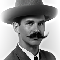

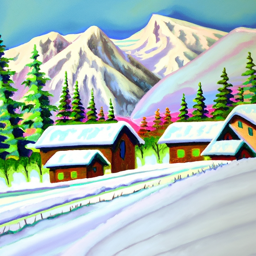
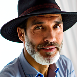
Firstly three images were sampled using seed = 45 with the text prompts in the captions. First 20 interference
steps were used and then 50. The quality of the images were not really affected in my opinion, maybe the second image of
a man wearing a hat is slightly more realistic.



In this part sampling loops were written by using the pre-trained DeepFloyd denoisers.
The forward process adds noise to a clean image x_0 to produce a noisy image x_t at
timestep t:
Noise increases with t, controlled by \alpha_t. Show results for
t = [250, 500, 750]. The original image is displyed down below and thereafter the noised images.


Classical denoising was implemented by applying Gaussian blur to the noisy images. The images were processed
for t = [250, 500, 750], and the results are displayed below.


I used a pretrained diffusion model to denoise the images. The denoiser, implemented as stage_1.unet,
is a UNet trained on a large dataset of image pairs. It recovers the Gaussian noise from the noisy image and removes
it to approximate the original image.


I created strided_timesteps, a list of monotonically decreasing timesteps starting at 990, with a stride of 30, and ending at 0. The timesteps were initialized using the function stage_1.scheduler.set_timesteps(timesteps=strided_timesteps).
The noisy image was displayed every 5th iteration of the denoising process, showing a gradual reduction in noise. The final predicted clean image was obtained using iterative denoising and displayed alongside comparisons to the results of single-step denoising, which appeared much worse, and Gaussian blurring from part 1.2.


Images were generated from scratch using a diffusion model by denoising random noise. Random noise tensors were
created with torch.randn and processed through the iterative_denoise function. The prompt
embedding "a high quality photo" guided the generation, producing five different images.


Classifier-Free Guidance (CFG) was used to improve image quality by combining conditional and unconditional noise
estimates with a scaling factor, γ, set to 7. The iterative_denoise_cfg function was
implemented to denoise images using both a prompt embedding for "a high quality photo" and an empty prompt embedding
for unconditional guidance. At each timestep, the UNet model was run twice to compute the conditional and unconditional
noise estimates, which were combined using the CFG formula. This process was repeated five times, producing images with
significantly enhanced quality compared to the previous part.


I applied the iterative_denoise_cfg function to the test image, adding noise and then denoising it with
starting indices of [1, 3, 5, 7, 10, 20]. The denoising process was guided by the prompt "a high quality photo" and
used a CFG scale of 7. To explore the method further, I repeated this process on two additional test images, demonstrating
its versatility. Noteworthy is that the model tended to generate images featuring women, even when the original content
was unrelated.


The same was done but this time for a non-realistic image where the first one if from the internet and the second two were drawn by me.s


This function uses a binary mask to keep the original image in unmasked areas while filling in masked regions with new content through iterative denoising. I tested it by inpainting the top of the Campanile in the test image and also worked on two custom images with different masks.


For this step, I used the text prompt "a rocket ship" to shape how the image changed during denoising. By starting at various noise levels [1, 3, 5, 7, 10, 20], the process mixed rocket-themed details into the original image. This was also done for two other images.


In this part the UNet model was run twice: once to denoise the image normally and then to denoise it flipped upside down. This allowed me to create an image that shows one scene when viewed right side up and a different scene when flipped. Using the prompts in the captions below visual anagrams were created.


To create hybrid images, I adapted the previous approach by combining the denoised high-frequency image with the denoised low-frequency image instead of summing the normal and flipped denoised images. This method makes the high-frequency details visible up close and the low-frequency content visible from a distance. Using the following prompts yielded three different images: "a lithograph of waterfalls" and "a lithograph of a skull", "a lithograph of a skull" and "a photo of a dog" and "a rocket ship" and "an oil painting of people around a campfire".


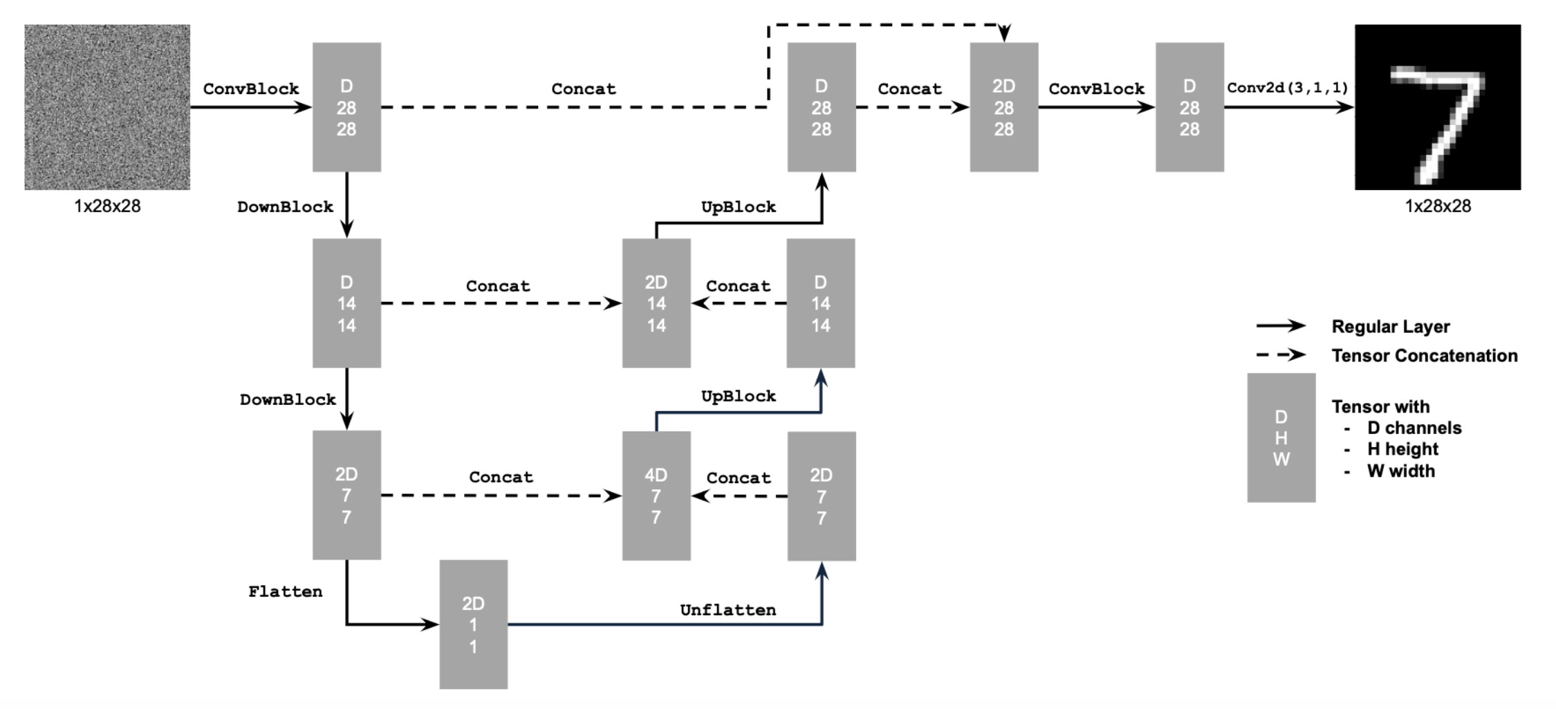
First the unconditioned UNet was implemented in accordance with the specifications presented down below.
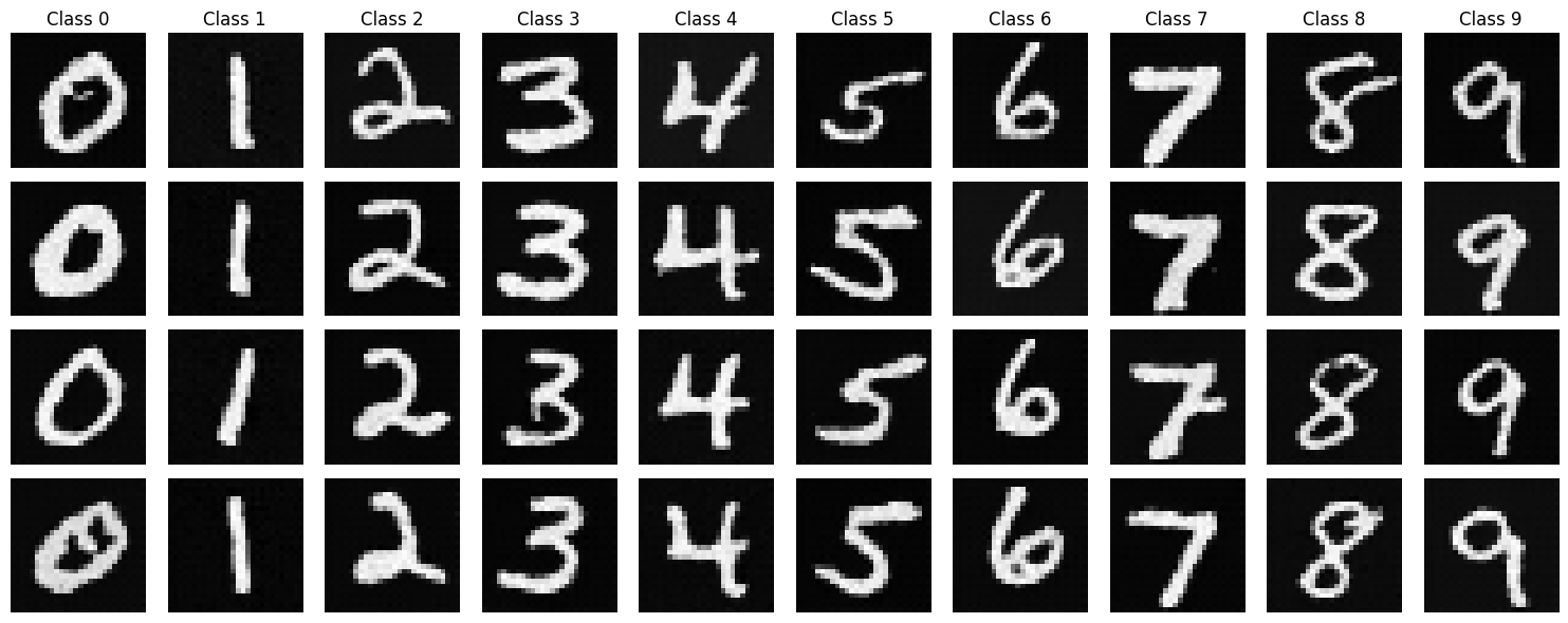
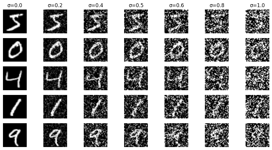
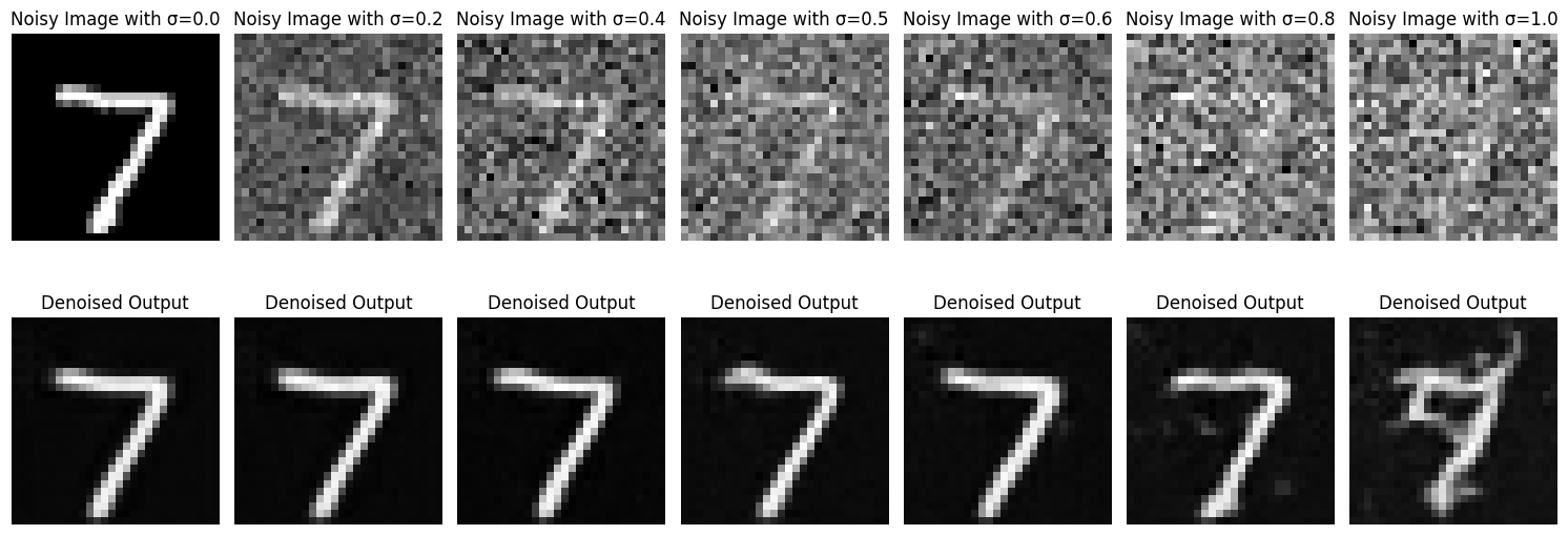
To train the model on MNIST, I first added varying levels of noise to the images for the model to learn from. The noise levels used were [0.0, 0.2, 0.4, 0.5, 0.6, 0.8, 1.0]. To illustrate the effect of the noise, I plotted five digits at each noise level. The results are shown below.
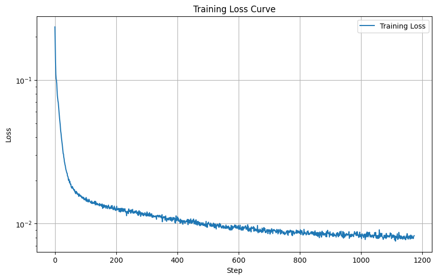
For training, I used image-class pairs with a batch size of 256, 5 epochs, \( \sigma = 0.5 \), and the Adam optimizer set to a learning rate of 1e-3. The training loss is shown below.
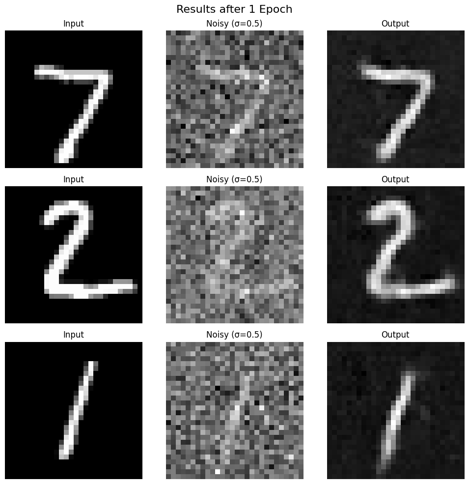
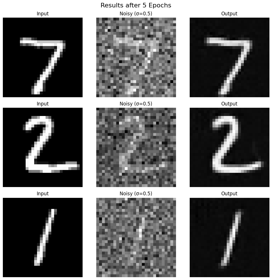
The results from the training are shown down below. First for after one epoch and then after five.
The model was trained on digits denoised with \( \sigma = 0.5 \). Below are the results when the denoiser is used on digits with different levels of noise.
In this section, a UNet model was trained to iteratively denoise images by predicting the noise added during the diffusion process. Instead of mapping a noisy image \( z \) back to a clean image \( x \), the UNet predicted the noise \( \epsilon \), as given by:
\[ L = \mathbb{E}_{\epsilon, z} \| \epsilon_\theta(z) - \epsilon \|^2, \]
where \( z = x + \sigma \epsilon \), and \( \epsilon \sim \mathcal{N}(0, I) \).
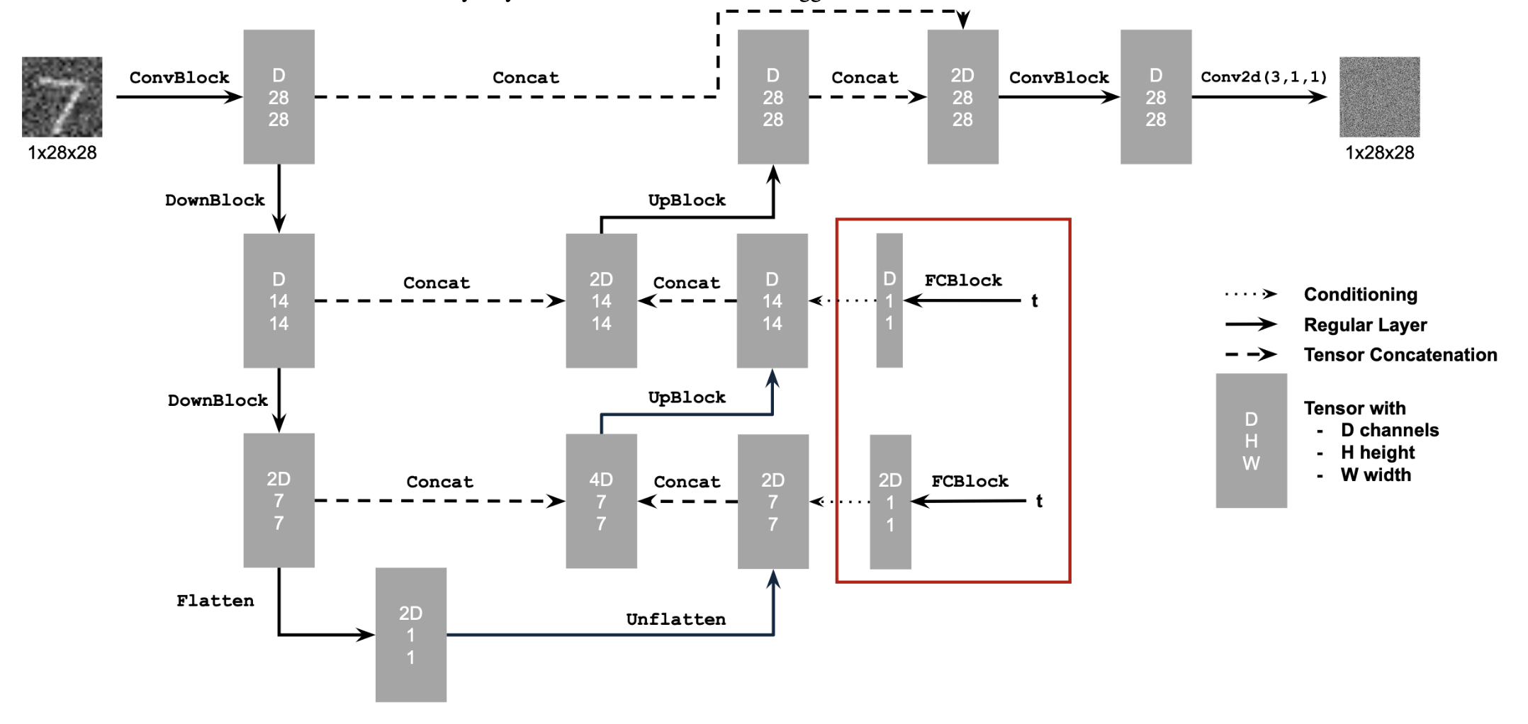
Time conditioning was introduced by embedding a normalized timestep \( t \) into the UNet using fully connected (FC) blocks. It was implemented in accordance with the schematic below.
The UNet was trained with the algorithm presented below.

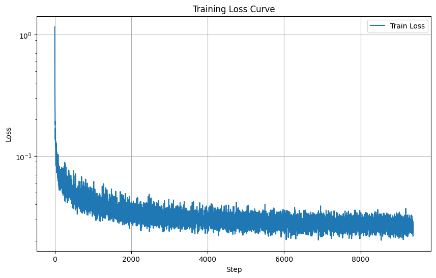
The training loss curve for the UNet is displayed below.
The results from using the time conditioned UNet is displayed down below, both for 5 and 20 epochs.
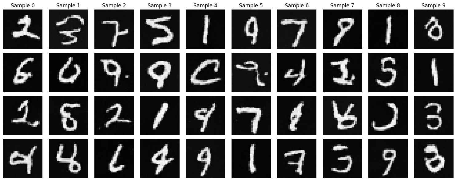

Lastly the Class-Conditioned UNet was implemented, conditioning the model on the class of the digit to be generated. This was achieved by adding two fully connected blocks to the UNet, using a one-hot encoded class label \( c \) as input. The training algorithm is presented down below.
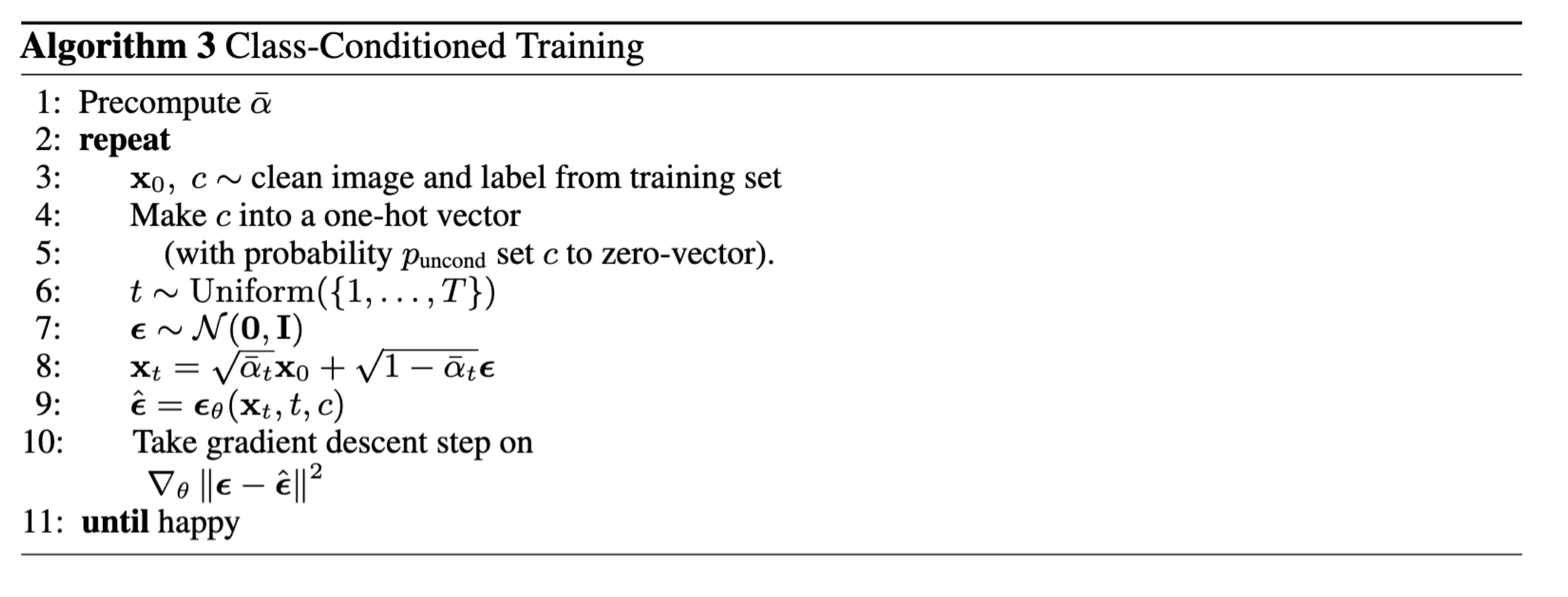
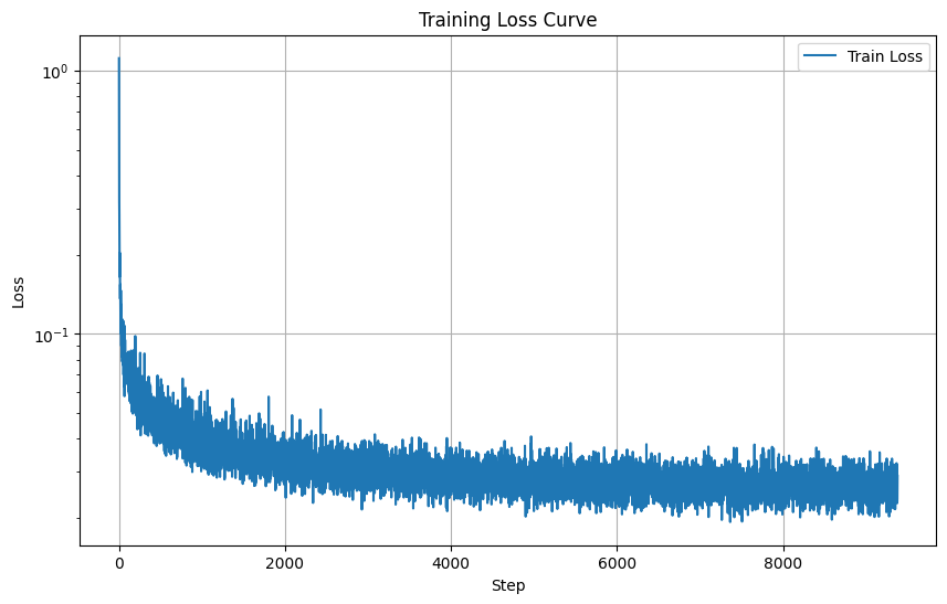
The training loss curve for this UNet is displayed below.
The results from this last UNet are presented down below, both after 5 epochs and after 20.
